R Practice 2

1 Tipos de datos

x <- 28
print(class(x))
y <- "R is fantastic"
print(class(y))
z <- TRUE
print(class(z))


[1] "numeric"

[1] "character"

[1] "logical"

1.1 Vectores

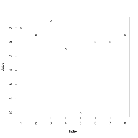
datos <- c(2,1,3,-1,-10,0,0,1)
print(datos)


[1]   2   1   3  -1 -10   0   0   1

1.1.1 Number sequences

print(1:10)
print(seq(10))
print(seq(1, 10, by=3))
print(rep(1:4, 2))

 [1]  1  2  3  4  5  6  7  8  9 10

 [1]  1  2  3  4  5  6  7  8  9 10

[1]  1  4  7 10

[1] 1 2 3 4 1 2 3 4

1.1.2 Access

print(datos)
print(datos[1])
print(datos[-4])
print(datos[c(1,3,5)])
print(datos[3:5])
print(v <- datos>1)
print(datos[v])

[1]   2   1   3  -1 -10   0   0   1

[1] 2

[1]   2   1   3 -10   0   0   1

[1]   2   3 -10

[1]   3  -1 -10

[1]  TRUE FALSE  TRUE FALSE FALSE FALSE FALSE FALSE

[1] 2 3

1.1.3 Index names

Vectors can have names on their indexes.

v = seq(1:5)
names(v) <- c("Lun", "Mar", "Mie", "Jue", "Vie")
print(v)

print(names(v))


Lun Mar Mie Jue Vie 
  1   2   3   4   5

[1] "Lun" "Mar" "Mie" "Jue" "Vie"

1.1.4 Fncs.

If a function does not return anything, then the vector may have a NA value.

print(length(datos))
print(min(datos))
print(max(datos))
print(sum(datos))
print(mean(datos))
print(median(datos))
print(sort(datos))
print(unique(datos))
print(which(datos > 1))
print(which.max(datos))
print(which.min(datos))

[1] 8

[1] -10

[1] 3

[1] -4

[1] -0.5

[1] 0.5

[1] -10  -1   0   0   1   1   2   3

[1]   2   1   3  -1 -10   0

[1] 1 3

[1] 3

[1] 5

plot(datos)

1.1.5 Factor

Nominal (unordered) or categorical (ordered) factor.

Used on Likert scale.

day_vector <- c('evening', 'morning', 'afrernoon', 'midday', 'midnight', 'evening')

factor_day <- factor(day_vector, order=TRUE, levels=c('morning', 'midday',
  'afternoon', 'evening', 'midnight'))

color_vector <- c('blue', 'red', 'yellow', 'green', 'white')

factor_color <- factor(color_vector)
print(factor_color)


[1] blue   red    yellow green  white 
Levels: blue green red white yellow

1.2 Data Frame

A new data frame can be created by using data.frame function.

a <- c(10, 20, 30 , 40)
b <- c('book', 'pen', 'textbook', 'pencil_case')
c <- c(TRUE, FALSE, TRUE, FALSE)
d <- c(2.5, 8, 10, 7)

df <- data.frame(a, b, c, d)
print(df)


   a           b     c    d
1 10        book  TRUE  2.5
2 20         pen FALSE  8.0
3 30    textbook  TRUE 10.0
4 40 pencil_case FALSE  7.0

Change names on the data frame.

names(df) <- c("ID", "items", "store", "price")
print(df)


  ID       items store price
1 10        book  TRUE   2.5
2 20         pen FALSE   8.0
3 30    textbook  TRUE  10.0
4 40 pencil_case FALSE   7.0

Print the structure and description of the data frame.

str(df)

'data.frame':	4 obs. of  4 variables:
 $ ID   : num  10 20 30 40
 $ items: Factor w/ 4 levels "book","pen","pencil_case",..: 1 2 4 3
 $ store: logi  TRUE FALSE TRUE FALSE
 $ price: num  2.5 8 10 7

1.2.1 Slices

print(df[1,2])
print(df[1:2,])
print(df[1:3, 3:4])
print(df[,1])
print(df[,"ID"])

[1] book
Levels: book pen pencil_case textbook

  ID items store price
1 10  book  TRUE   2.5
2 20   pen FALSE   8.0

  store price
1  TRUE   2.5
2 FALSE   8.0
3  TRUE  10.0

[1] 10 20 30 40

[1] 10 20 30 40

1.2.2 Add columns

The amount of data in the vector must be of the same length of the data frame's columns.

quantity <- c(10, 35, 40, 5)

df$quantity <- quantity

print(df)


  ID       items store price quantity
1 10        book  TRUE   2.5       10
2 20         pen FALSE   8.0       35
3 30    textbook  TRUE  10.0       40
4 40 pencil_case FALSE   7.0        5

1.2.3 Subset

print(subset(df, subset=price > 5))

  ID       items store price quantity
2 20         pen FALSE     8       35
3 30    textbook  TRUE    10       40
4 40 pencil_case FALSE     7        5

1.2.4 Merge - Joins

Full merge is when both columns has data. Partial merge is when one of the column has data that is not in the other, then a NA value will be assigned.

x <- c("n1", "n2")
y <- c(1, 2)
z <- data.frame(x, y)

print(z)

t <- c("a", "b")
s <- c(1, 2)
o <- data.frame(t, s)

print(o)

q <- merge(z, o, by.x = "y", by.y = "s")
print(q)


   x y
1 n1 1
2 n2 2

  t s
1 a 1
2 b 2

  y  x t
1 1 n1 a
2 2 n2 b

Partial match. The following snippet adds a new row into z.

add_z <- c("n2", 3)
z <- rbind(z, add_z)

print(z)

# Partial match
q <- merge(z, o, by.x = "y", by.y = "s", all.x = TRUE)
print(q)

# Total  match 
q <- merge(z, o, by.x = "y", by.y = "s")
print(q)


   x y
1 n1 1
2 n2 2
3 n2 3

  y  x    t
1 1 n1    a
2 2 n2    b
3 3 n2 <NA>

  y  x t
1 1 n1 a
2 2 n2 b

2 Plotting

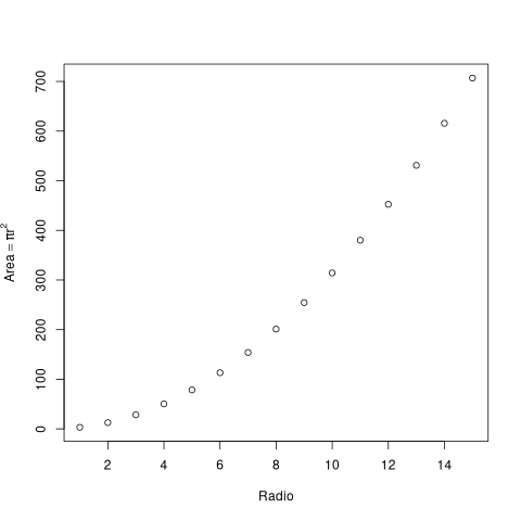
x <- 1:15
y <- pi*x^2

print(x)
print(y)


 [1]  1  2  3  4  5  6  7  8  9 10 11 12 13 14 15

 [1]   3.141593  12.566371  28.274334  50.265482  78.539816 113.097336
 [7] 153.938040 201.061930 254.469005 314.159265 380.132711 452.389342
[13] 530.929158 615.752160 706.858347

plot(x, y, xlab="Radio", ylab=expression(Area == pi*r^2))

Correlation. If p-value < 0.05, then they are correlated. If cor is near 1, the more correlated they are.

res <- cor.test(x,y)
print(res)


	Pearson's product-moment correlation

data:  x and y
t = 15.029, df = 13, p-value = 1.348e-09
alternative hypothesis: true correlation is not equal to 0
95 percent confidence interval:
 0.9168624 0.9910175
sample estimates:
      cor 
0.9724093

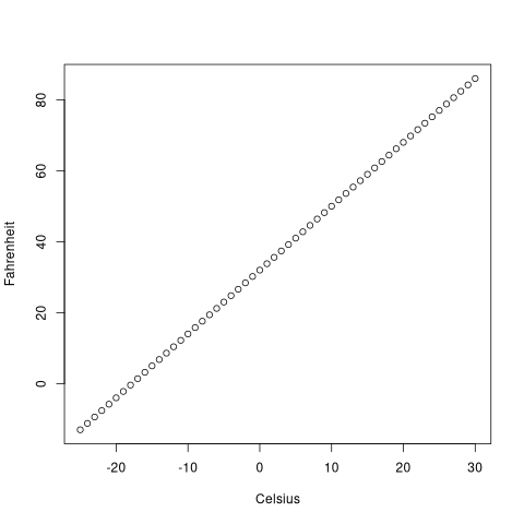
celsius <- -25:30
fahrenheit <- 9/5*celsius+32
x <- data.frame(Celsius=celsius, Fahrenheit=fahrenheit)
plot(x)

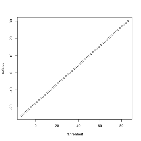
plot(celsius~fahrenheit)

2.1 Bar plot

library(MASS)
t <- table(survey$Sex, survey$Smoke)
print(t)



       Heavy Never Occas Regul
Female     5    99     9     5
Male       6    89    10    12

barplot(table(survey$Sex, survey$Smoke), beside=TRUE)

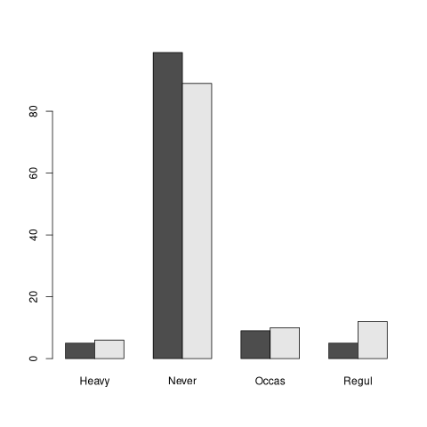
barplot(t, beside=TRUE)

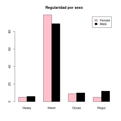
barplot(t, main="Regularidad por sexo", legend.text=c("Female", "Male"),
  beside=TRUE, col = c("pink", "black"))

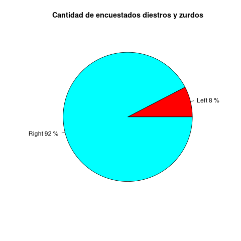
2.2 Pie plot

f <- table(survey$Sex)
print(f)


Female   Male 
   118    118

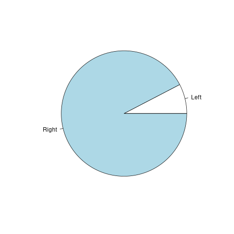
f <- table(survey$W.Hnd)
print(f)


Left Right 
  18   218

pie(f)

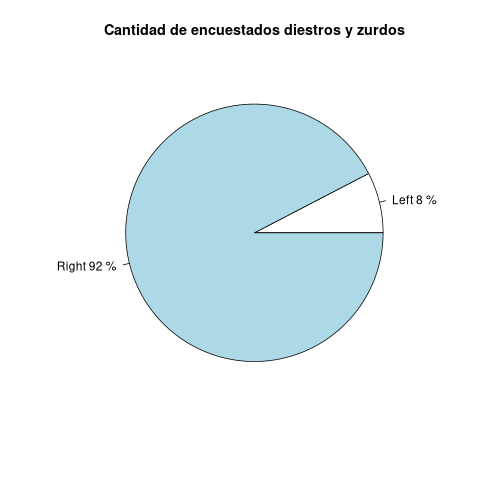
z <- round(f/sum(f)*100)

print(z)
lbs <- paste(names(f), z, "%", sep=" ")
print(lbs)


 Left Right 
    8    92

[1] "Left 8 %"   "Right 92 %"

pie(f, main="Cantidad de encuestados diestros y zurdos", labels=lbs)

pie(f, main="Cantidad de encuestados diestros y zurdos", labels=lbs,
  col=rainbow(length(lbs)))

2.3 Histograms

hist(survey$Age)

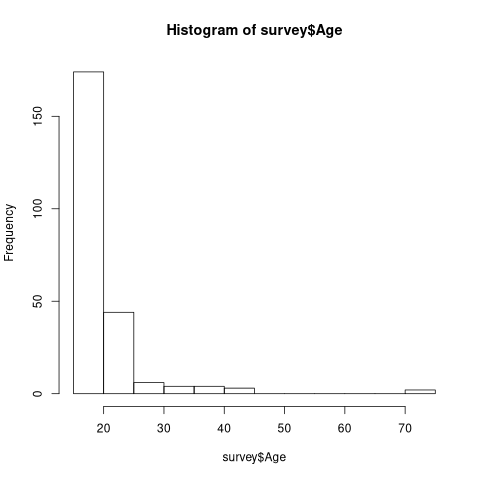
This is a normal distributed histogram.

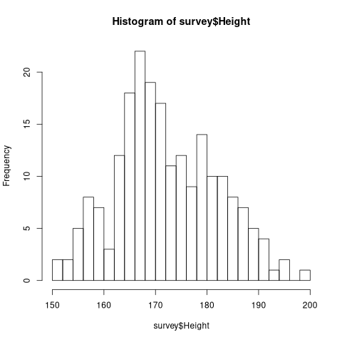
hist(survey$Height)

Testing normality.

print(shapiro.test(survey$Age))


	Shapiro-Wilk normality test

data:  survey$Age
W = 0.45642, p-value < 2.2e-16

If p-value > 0.05 then it is normal.

print(shapiro.test(survey$Height))


	Shapiro-Wilk normality test

data:  survey$Height
W = 0.98841, p-value = 0.08844

2.3.1 Example

#........................................Histograma

tiempo <- c(11.50 , 10.26, 10.08, 13.00, 11.14, 13.73, 13.41, 10.44, 11.36, 14.40, 11.64, 12.39, 12.82, 14.25, 15.41, 14.35, 9.35, 12.40, 9.04, 15.30, 14.79, 15.27, 10.63, 14.30, 15.48, 14.80, 8.78, 14.00, 13.09, 10.00, 12.20, 11.70, 15.37, 11.81, 10.06, 12.49, 8.58, 11.32, 12.20, 12.45, 11.28, 12.60, 14.36, 13.08, 13.50, 12.68, 9.19, 14.32, 12.17, 9.10)
sum <- min(tiempo)
for (i in 1:7) { 
  sum <- sum + 0.99 
  print(sum) }

#........................................Barplot 

x <- c(rep("muy de acuerdo",10), rep("de acuerdo", 10), rep("poco de acuerdo", 10), rep("para nada de acuerdo", 10))

factor_x <- factor(x, order=TRUE, levels = c("para nada de acuerdo", "poco de acuerdo", "de acuerdo", "muy de acuerdo"))
w <- as.numeric(factor_x)

y <- c(rep("hombre",18), rep("mujer",2), rep("mujer",18), rep("hombre",2))


#........................................Boxplot
g <- c(36,25,37,24,39,20,36,45,31,31,39,24,29,23,41,40,33,24,34,40)
g


[1] 9.57
[1] 10.56
[1] 11.55
[1] 12.54
[1] 13.53
[1] 14.52
[1] 15.51

 [1] 36 25 37 24 39 20 36 45 31 31 39 24 29 23 41 40 33 24 34 40

tiempo <- c(11.50 , 10.26, 10.08, 13.00, 11.14, 13.73, 13.41, 10.44, 11.36, 14.40, 11.64, 12.39, 12.82, 14.25, 15.41, 14.35, 9.35, 12.40, 9.04, 15.30, 14.79, 15.27, 10.63, 14.30, 15.48, 14.80, 8.78, 14.00, 13.09, 10.00, 12.20, 11.70, 15.37, 11.81, 10.06, 12.49, 8.58, 11.32, 12.20, 12.45, 11.28, 12.60, 14.36, 13.08, 13.50, 12.68, 9.19, 14.32, 12.17, 9.10)

11.5
10.26
10.08
13
11.14
13.73
13.41
10.44
11.36
14.4
11.64
12.39
12.82
14.25
15.41
14.35
9.35
12.4
9.04
15.3
14.79
15.27
10.63
14.3
15.48
14.8
8.78
14
13.09
10
12.2
11.7
15.37
11.81
10.06
12.49
8.58
11.32
12.2
12.45
11.28
12.6
14.36
13.08
13.5
12.68
9.19
14.32
12.17
9.1

trange <- range(tiempo)
tmax <- max(tiempo)
tmin <- min(tiempo)
print(trange)
trange2 <- tmax-tmin
print(trange2)


[1]  8.58 15.48

[1] 6.9

int_clase <- sqrt(length(tiempo))
print(int_clase)
int_clase <- round(int_clase)
print(int_clase)


[1] 7.071068

[1] 7

amplitud <- trange2/int_clase
print(amplitud)
amplitud <- round(amplitud)
print(amplitud)


[1] 0.9857143

[1] 1

The number of classes in a histogram can be changed with the nclass parameter.

hist(survey$Height, nclass=20)

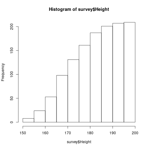
2.3.2 Acumulative (Frequent) Histograms

z$counts has the frequency of the elements in the histograms.

z <- hist(survey$Height)

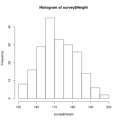
print(z$counts)

8
16
29
45
33
30
26
14
6
2

z$counts <- cumsum(z$counts)

print(z$counts)

8
24
53
98
131
161
187
201
207
209

plot(z)

2.4 Box Plot

g <- c(36,25,37,24,39,20,36,45,31,31,39,24,29,23,41,40,33,24,34,40)
bp1 <- boxplot(g)

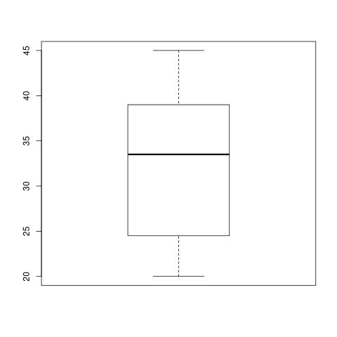
print(bp1)

$stats
     [,1]
[1,] 20.0
[2,] 24.5
[3,] 33.5
[4,] 39.0
[5,] 45.0

$n
[1] 20

$conf
         [,1]
[1,] 28.37717
[2,] 38.62283

$out
numeric(0)

$group
numeric(0)

$names
[1] "1"

horizontal plot

bp2 <- boxplot(g, horizontal=TRUE)

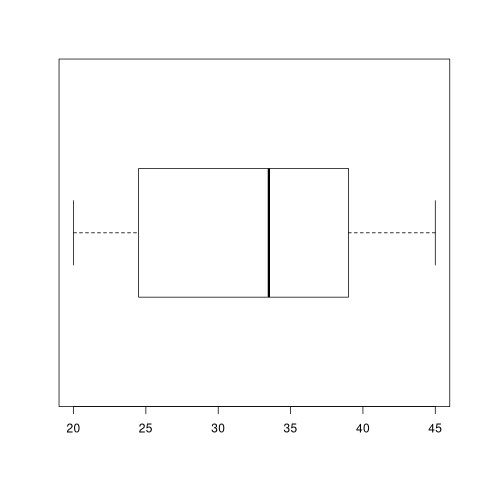
print(bp2)

$stats
     [,1]
[1,] 20.0
[2,] 24.5
[3,] 33.5
[4,] 39.0
[5,] 45.0

$n
[1] 20

$conf
         [,1]
[1,] 28.37717
[2,] 38.62283

$out
numeric(0)

$group
numeric(0)

$names
[1] "1"

bp1$stats returns the quartiles values.

print(sort(g))

print(bp1$stats)

 [1] 20 23 24 24 24 25 29 31 31 33 34 36 36 37 39 39 40 40 41 45

     [,1]
[1,] 20.0
[2,] 24.5
[3,] 33.5
[4,] 39.0
[5,] 45.0

2.4.1 Quartiles

g1 <- sort(g)
print(g1)


[1] 20 23 24 24 24 25 29 31 31 33 34 36 36 37 39 39 40 40 41 45

First quartile is the arithmetic media between the 4th quarter and the next values.

print(
  (g1[length(g1)/4] + g1[length(g1)/4 + 1] ) / 2
)


[1] 24.5

print(median(g1))

[1] 33.5

3 Correlation

print(min(survey$NW.Hnd, na.rm=TRUE))

[1] 12.5

plot(survey$Wr.Hnd, survey$NW.Hnd)

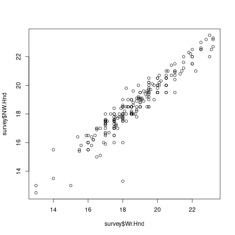
res <- cor.test(survey$Wr.Hnd, survey$NW.Hnd)
print(res)


	Pearson's product-moment correlation

data:  survey$Wr.Hnd and survey$NW.Hnd
t = 45.712, df = 234, p-value < 2.2e-16
alternative hypothesis: true correlation is not equal to 0
95 percent confidence interval:
 0.9336780 0.9597816
sample estimates:
      cor 
0.9483103

To ensure that the Pearson method is applied, use the method parameter.

res <- cor.test(survey$Wr.Hnd, survey$NW.Hnd, method="pearson")
print(res)


	Pearson's product-moment correlation

data:  survey$Wr.Hnd and survey$NW.Hnd
t = 45.712, df = 234, p-value < 2.2e-16
alternative hypothesis: true correlation is not equal to 0
95 percent confidence interval:
 0.9336780 0.9597816
sample estimates:
      cor 
0.9483103

3.1 Wilcox correlation

Some comparison between a Likert (nominal) with another factor it has to be applied with the corresponding parametric or non-parametric correlation.

x <- c(rep("muy de acuerdo",10), rep("de acuerdo", 10), rep("poco de acuerdo", 10), rep("para nada de acuerdo", 10))
factor_x <- factor(x, order=TRUE, levels = c("para nada de acuerdo", "poco de acuerdo", "de acuerdo", "muy de acuerdo"))
print(factor_x)

w <- as.numeric(factor_x)
print(w)

y <- c(rep("hombre",18), rep("mujer",2), rep("mujer",18), rep("hombre",2))
print(y)


 [1] muy de acuerdo       muy de acuerdo       muy de acuerdo      
 [4] muy de acuerdo       muy de acuerdo       muy de acuerdo      
 [7] muy de acuerdo       muy de acuerdo       muy de acuerdo      
[10] muy de acuerdo       de acuerdo           de acuerdo          
[13] de acuerdo           de acuerdo           de acuerdo          
[16] de acuerdo           de acuerdo           de acuerdo          
[19] de acuerdo           de acuerdo           poco de acuerdo     
[22] poco de acuerdo      poco de acuerdo      poco de acuerdo     
[25] poco de acuerdo      poco de acuerdo      poco de acuerdo     
[28] poco de acuerdo      poco de acuerdo      poco de acuerdo     
[31] para nada de acuerdo para nada de acuerdo para nada de acuerdo
[34] para nada de acuerdo para nada de acuerdo para nada de acuerdo
[37] para nada de acuerdo para nada de acuerdo para nada de acuerdo
[40] para nada de acuerdo
4 Levels: para nada de acuerdo < poco de acuerdo < ... < muy de acuerdo

 [1] 4 4 4 4 4 4 4 4 4 4 3 3 3 3 3 3 3 3 3 3 2 2 2 2 2 2 2 2 2 2 1 1 1 1 1 1 1 1
[39] 1 1

 [1] "hombre" "hombre" "hombre" "hombre" "hombre" "hombre" "hombre" "hombre"
 [9] "hombre" "hombre" "hombre" "hombre" "hombre" "hombre" "hombre" "hombre"
[17] "hombre" "hombre" "mujer"  "mujer"  "mujer"  "mujer"  "mujer"  "mujer" 
[25] "mujer"  "mujer"  "mujer"  "mujer"  "mujer"  "mujer"  "mujer"  "mujer" 
[33] "mujer"  "mujer"  "mujer"  "mujer"  "mujer"  "mujer"  "hombre" "hombre"

The Wilcoxon test has a p-value less than 0.05 which means that there is correlation between the Likert data (w or x) that is influenced by the sex (y data).

m <- data.frame(w, y)
wilcox.test(w~y, alternative="two.sided", data=m)
print(m)


	Wilcoxon rank sum test with continuity correction

data:  w by y
W = 360, p-value = 8.405e-06
alternative hypothesis: true location shift is not equal to 0

Warning message:
In wilcox.test.default(x = c(4, 4, 4, 4, 4, 4, 4, 4, 4, 4, 3, 3,  :
  cannot compute exact p-value with ties

   w      y
1  4 hombre
2  4 hombre
3  4 hombre
4  4 hombre
5  4 hombre
6  4 hombre
7  4 hombre
8  4 hombre
9  4 hombre
10 4 hombre
11 3 hombre
12 3 hombre
13 3 hombre
14 3 hombre
15 3 hombre
16 3 hombre
17 3 hombre
18 3 hombre
19 3  mujer
20 3  mujer
21 2  mujer
22 2  mujer
23 2  mujer
24 2  mujer
25 2  mujer
26 2  mujer
27 2  mujer
28 2  mujer
29 2  mujer
30 2  mujer
31 1  mujer
32 1  mujer
33 1  mujer
34 1  mujer
35 1  mujer
36 1  mujer
37 1  mujer
38 1  mujer
39 1 hombre
40 1 hombre

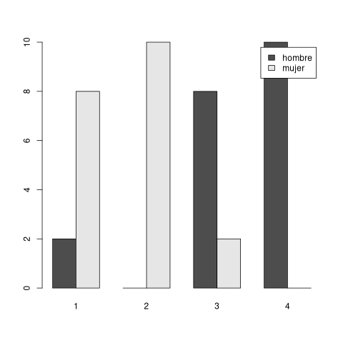
barplot(table(m), beside=TRUE, legend=TRUE)

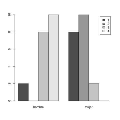
barplot(table(y, w), beside=TRUE, legend=TRUE)

4 License of This Work

This work is licensed under the Creative Commons Attribution-NoDerivatives 4.0 International License. To view a copy of this license, visit http://creativecommons.org/licenses/by-nd/4.0/.

R Practice 2 by Gimenez Christian is licensed under a Creative Commons Attribution-NoDerivatives 4.0 International License.