R Practice 3
1 Variables
- Dependent
- Attractiveness
- Independent
- 3 Factors
- No alcohol
- 2 pints
- 4 pints
2 dataset Package
WRS2 provides a dataset called goggles. The following code loads the package, loads the goggles dataframe and shows its first rows.
library(WRS2)
data(goggles)
head(goggles)
  gender alcohol attractiveness
1 Female    None             65
2 Female    None             70
3 Female    None             60
4 Female    None             60
5 Female    None             60
6 Female    None             55
summary shows some information about the dataframe fields.
summary(goggles)
   gender      alcohol   attractiveness
Female:24   None   :16   Min.   :20.00
Male  :24   2 Pints:16   1st Qu.:53.75
            4 Pints:16   Median :60.00
                         Mean   :58.33
                         3rd Qu.:66.25
                         Max.   :85.00
3 psych
psych package provides the describeBy function which shows more details about the relation between two fields.
First, the following loads the package.
library(psych)
Secondly, it shows the relation between attractiveness according to the amount of alcohol drinked. The results is grouped between the three possible values of the alcohol domain.
describeBy(goggles$attractiveness, goggles$alcohol)
 Descriptive statistics by group
group: None
   vars  n  mean   sd median trimmed   mad min max range skew kurtosis   se
X1    1 16 63.75 8.47   62.5   63.57 11.12  50  80    30 0.29    -1.07 2.12
------------------------------------------------------------
group: 2 Pints
   vars  n  mean   sd median trimmed  mad min max range skew kurtosis   se
X1    1 16 64.69 9.91     65   64.64 7.41  45  85    40 0.08    -0.23 2.48
------------------------------------------------------------
group: 4 Pints
   vars  n  mean    sd median trimmed   mad min max range  skew kurtosis   se
X1    1 16 46.56 14.34     50   46.79 14.83  20  70    50 -0.22    -1.21 3.59
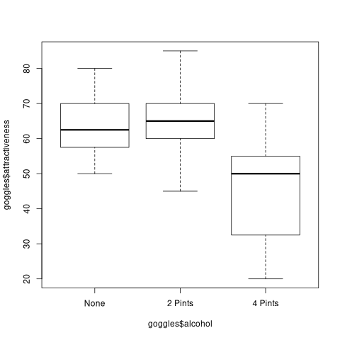
4 Plotting
Plotting can be done by the plot function or one of their most specific one. boxplot creates a box plot which shows the relation between attractiveness (Y axis) and alcohol (X axis).
boxplot(goggles$attractiveness ~ goggles$alcohol)
5 Outlier values
The rapportools package provides the rp.outlier functions. It search for all extreme values. Use help(rp.outlier) for more information about the method used.
library(rapportools)
a <- rp.outlier(goggles[goggles$alcohol == "None",  "attractiveness"])
print(a)
b <- rp.outlier(goggles[goggles$alcohol == "2 Pints", "attractiveness"])
print(b)
c <- rp.outlier(goggles[goggles$alcohol == "4 Pints", "attractiveness"])
print(c)
NULL

NULL

NULL
6 Test for Anova Requirements
Before using the Anova, some requirements must be met. The following section shows how to test for normality of their data and homoscedasticity (variance homogeneity).
6.1 Normalidad
The Shapiro-Wilk test for normality on the data. If the p-value is greater than 0.05, it implies that distribution of the data is not significantly different from a normal distribution.
by(goggles$attractiveness, goggles$alcohol, shapiro.test)
goggles$alcohol: None

	Shapiro-Wilk normality test

data:  dd[x, ]
W = 0.95498, p-value = 0.5725

------------------------------------------------------------
goggles$alcohol: 2 Pints

	Shapiro-Wilk normality test

data:  dd[x, ]
W = 0.94489, p-value = 0.4132

------------------------------------------------------------
goggles$alcohol: 4 Pints

	Shapiro-Wilk normality test

data:  dd[x, ]
W = 0.952, p-value = 0.522
6.2 TODO Homoscedasticity or variances homogeneity
A set of variables is homoscedastic if all of them have the same finite variance. The following are example codes that apply the Barlett, Levene and Fligner tests.
bartlett.test(goggles$attractiveness, goggles$alcohol)
library(car)
leveneTest(goggles$attractiveness, goggles$alcochol)
fligner.test(goggles$attractivess, goggles$alcohol)
7 Anova
Once the homoscedaticity and normal distribution of data are confirmed, the Anova analisys can be applied.
The following code execute the Anova and display the results.
analysis <- aov(attractiveness ~ alcohol, data=goggles)
summary(analysis)
            Df Sum Sq Mean Sq F value   Pr(>F)
alcohol      2   3332  1666.1   13.31 2.88e-05 ***
Residuals   45   5634   125.2
---
Signif. codes:  0 ‘***’ 0.001 ‘**’ 0.01 ‘*’ 0.05 ‘.’ 0.1 ‘ ’ 1
7.1 Which one?
aov does not show which are the groups related. TukeyHSD display grouped with the different factors the p-value of their relation. A p-value less than 0.05 means that there are sifnificantly difference between the factors.
TukeyHSD(analysis)
  Tukey multiple comparisons of means
    95% family-wise confidence level

Fit: aov(formula = attractiveness ~ alcohol, data = goggles)

$alcohol
                    diff        lwr       upr     p adj
2 Pints-None      0.9375  -8.650654 10.525654 0.9695381
4 Pints-None    -17.1875 -26.775654 -7.599346 0.0002283
4 Pints-2 Pints -18.1250 -27.713154 -8.536846 0.0001067
8 License of This Work
This work is licensed under the Creative Commons Attribution-NoDerivatives 4.0 International License. To view a copy of this license, visit http://creativecommons.org/licenses/by-nd/4.0/.

R Practice 3 by Gimenez Christian is licensed under a Creative Commons Attribution-NoDerivatives 4.0 International License.